3.1.A1. Methodology of assessment of water-related ES
General modeling framework
Four of the six regulating services assessed are closely linked to the water cycle via evapotranspiration and indicators of surface runoff and baseflow. They were assessed using the InVEST (Integrated Valuation of Ecosystem Services and Tradeoffs) integrated tool:
– Seasonal water flow regulation and baseflow provision (InVEST Seasonal Water Yield);
– Prevention of soil water erosion and sediment export in waterbodies (InVEST Sediment Delivery Ratio);
– Ջրհեղեղի ռիսկի նվազեցում (InVEST Urban Flood Risk Mitigation);
– Ցամաքային էկոհամակարգերի սառեցնող ազդեցությունը (InVEST Urban Cooling).
The modeling framework simulated current (2023) and past (2017) conditions, as well as alternative land-cover scenarios, to evaluate ecosystem services (ES) provided by terrestrial ecosystems and to detect changes in these services (Figure 31A1-1). To calculate ES values across the different EAAs, we used the administrative boundary map from the Forest Atlas of Armenia and the vegetation map developed under the project (Section 2.3). A comparison of the modeling results with ARMSTAT water-use data was conducted to assess the supply–use balance, thereby demonstrating the relevance of ES accounting data for evidence-based decision-making on water use and territorial development.
Figure 31A1-1. Flow-chart of ES assessment.
The InVEST models used
The ES of seasonal water flow regulation and baseflow provision was estimated and mapped with InVEST Seasonal Water Yield (SWY) model which estimates the impact of terrestrial ecosystems on the total amount of water flow and its seasonal redistribution. Based on monthly precipitation, reference evapotranspiration, soil permeability, topography, and the land use/land cover (LULC), the model calculates two key indicators: quick flow and baseflow. Quick flow represents the portion of precipitation that runs off during or shortly after a rain event (within hours to days). Baseflow is the portion of precipitation that gradually enters streams through subsurface flow with watershed residence times ranging from months to years. Baseflow plays a crucial role in maintaining water flow during dry periods and mitigating the impacts of drought.
The ES of prevention of soil water erosion and sediment export in waterbodies was estimated and mapped with InVEST Sediment Delivery Ratio (SDR) model which estimates the impact of terrestrial ecosystems on soil water erosion and sediment export into streams. The model relies on the widely used Universal Soil Loss Equation (USLE) and Sediment Delivery Ratio that estimates the ratio between the amount of sediment eroded from each land pixel, the amount of sediment that is trapped along the flow path downslope from this pixel, and the amount of sediment that reaches a stream. Based on rainfall erosivity, soil erodibility, topographic, and LULC data, the model calculates potential and avoided erosion and sediment export into streams. Thus, the model evaluates and maps two ecosystem services simultaneously: prevention of soil water erosion and ensuring water flow quality.
The ES of flood risk mitigation was estimated and mapped with InVEST Urban Flood Risk Mitigation (UFRM) model which calculates two main indicators: (1) the runoff retention, i.e., the amount of runoff retained by soil and vegetation when modeling rainfall; (2) the runoff (Q), mm, which is a potentially hazardous factor that can cause flooding. These calculations were based on LULC, soil hydrologic groups, watersheds and climate data.
Сooling effect of terrestrial ecosystems was estimated and mapped with InVEST Urban Cooling (UC) model which is primarily aimed at assessing the cooling effect of green spaces within urban areas. However, it also allows for evaluating this effect over large areas outside of cities. Since the assessment of urban ES is not a goal of our project, we focused on the ES of areas outside settlements. We used the Cooling Capacity Calculation Method, which estimates cooling capacity based on evapotranspiration, albedo, shade (the proportion of area that is covered by tree canopy), air temperature in a rural reference area, and the Urban Heat Index (UHI), i.e., the difference between the rural reference temperature and the maximum temperature observed in the city. We modeled this ES for the hottest season in Armenia—July and August.
Detailed descriptions of the models can be found in the above-mentioned sections of the InVEST website and in the InVEST User Guide [42].
Model inputs
Table 31A1-1. Model inputs
| Data Type | Models | Sources | Notes |
| LULC | SWY, SDR, UFRM, UC | ESRI land cover data [40] | Resolution 10 m Data for 2017 and 2023 |
| Soil hydrologic groups | SWY, UFRM | Soil map of Armenia from [38] | Vector map The hydrological soil groups were defined in accordance with USDA recommendations [44]: A—slightly and moderately stony sand; very stony sandy loam; B—slightly and moderately stony sandy loam; very stony loam; C—slightly and moderately stony loam; very stony clay; D—slightly and moderately stony clay. The obtained map of soil hydrologic groups is presented on the project’s webGIS [45] |
| Soil erodibility (K-factor) | SDR | Soil map of Armenia from [38] | Vector map A soil erodibility map was obtained on the basis of soil textures using the following coefficients from the InVEST User Guide [42]: 0.0290 for clay, 0.0395 for loam, 0.0171 for sandy loam, 0.0026 for sand. |
| Digital elevation model | SWY, SDR | [46] | Resolution 30 m |
| Watershed boundaries | SWY, SDR, UFRM | [39] | Vector map The analysis was made for parts of watersheds that are located on the territory of Armenia: Aghstev, Akhuryan, Arpa, Debed, Hrazdan, Metsamor, and Vorotan (Figure 1b) |
| Climate data (average annually and monthly precipitation and temperature) | SWY, UFRM< UC | [47] | Resolution 30 arc seconds * The amount of liquid precipitation has been adjusted to take into account the snow period (see below) |
| Rain events table | SWY, UFRM | [48] | The number of rainy days for each climatic zone was calculated as the average for several cities located within that zone. In the moderate-cool climate zone, where there are no cities, the average data for this zone is based on three cities situated near its border [49] |
| Climate zones of Armenia | SWY, SDR, UC, UFRM | The map of climate zones of Armenia from [38] | Vector map The digital vector map of climate zones of Armenia was generalized to the four climate zones: (1) Arid; (2) Moderate dry; (3) Moderate cool; (4) Moderate humid. For details, see the project’s webGIS [45] |
| Monthly reference evapotranspiration (ET0) | SWY, UC | [50] | Resolution 30 arc seconds * |
| Crop coefficients Kc | SWY, UC | [51,52] | Kc were determined for the four climate zones. The used Kc are presented at the project website [49] |
| Vegetation periods for crops | SWY, UC | [53] | Vegetation periods were determined for the four climate zones |
| Leaf Area Index | SWY, UC | [54] | The LAI values for dates in the middle of the months were used |
| Curve numbers (CN) | SWY, UFRM | [55–57] | Coefficients for medium hydrological conditions and medium vegetation states were used. For croplands and rangelands, differences in climatic zones were taken into account [48] |
| C-factor for crops | SDR | [58] | C-factor was defined as average values for Europe: 0.3 for crops and sparse vegetation, 0.05 for rangelands (average between pastures and low productive grasslands), and 0.0014 for forests (average value for Southern European countries). C-factor was considered equal to zero for water, flooded vegetation, built areas, and snow/ice on the InVEST recommendations. |
| P-factor | SDR | – | P-factor was considered equal to 1 because we did not take into account special anti-erosion measures |
| Rainfall erosivity | SDR | [59] | Resolution 30 arc seconds * |
| Albedo | UC | [58] | The following albedo values were used for land cover classes: water and flooded vegetation 0,6; trees 0.15; rangeland 0.2; crops 0.2; built-up area 0.17; bare ground 0.25; snow/ice 0.9 |
| Shade | UC | – | The following shade values were used for land cover classes: built-up – 0.2; forests – 1.0; croplands, taking into account the share of orchard area, in the arid climate zone – 0.35, in the moderate-dry and moderate-cool zones – 0.03, in the moderate-humid zone – 0.34, other land cover classes – 0. |
| UHI effect | UC | [59] | The UHI value was set to zero |
Crop coefficients (Kc) were defined as average values for the main groups of agricultural crops, based on FAO data [51,52]. Areas of various agricultural crops such as grains and legumes, vegetables, potatoes, melons, fruits and berries, and grapes in the provinces of Armenia in 2023 were obtained from the Statistical Committee of the Republic of Armenia [41]. To calculate Kc for croplands, we averaged the area shares of different crops for four climatic zones based on data from provinces predominantly located in one or another zone. Average Kc values were then calculated for croplands in each climatic zone, taking into account the share of the area of different agricultural crops within it. Kc values for bare soil were determined based on [60] as the average values for different soil types. For natural vegetation (rangeland and trees), in accordance with the recommendations of InVEST [42], Kc values were set as Kc = 1 if LAI > 3 and Kc = LAI/3 if LAI ≤ 3. According to InVEST and FAO [52] recommendations, Kc = 1 was used for water and flooded vegetation, Kc = 0.35—for built-up areas (assuming that impervious surfaces account for 50%), and Kc = 0.4—for permanent snow. The values of other coefficients were taken from the InVEST User Guide recommendations [42].
UHI effect is incorporated into UC model as a single value. Calculations based on a single UHI value for all of Armenia are impractical due to the significant variation in conditions across different cities. The global UHI effect map [59] shows that in Armenia, it has varying values with opposite signs in different settlements—some settlements are warmer than their surroundings, while others are colder, which makes the use of this factor biased [62]. Therefore, we decided not to account for this factor and set the UHI value to 0.
The values of other coefficients were taken from the InVEST User Guide recommendations [42].
Regional ArmStat statistics on water consumption in 2023 were used to estimate the consumption of ESs.
Scenarios used for ES modeling
To estimate the role of natural ecosystems in ES provisioning, we used three hypothetical LULC scenarios:
– Bare ground scenario: all vegetation, including forests and grasslands, was replaced with bare ground;
– Cropland scenario: all areas, except for urban territories and water bodies, were converted to cropland;
– No-human scenario: urban areas and croplands were replaced with grasslands, simulating a landscape without human activity.
One of the tested models—SDR—directly calculates ES values provided by ecosystems, i.e., indicators of avoided erosion and avoided sediment export. The other models calculate ES indicators for a given LULC but do not determine what portion of these values is attributable to ecosystems rather than to physical processes. In the SWY and UFRM models, we estimated the volume of ES provided by ecosystems as the difference between ES values for the current land cover and the bare ground scenario. The cropland scenario was used in the SWY model to compare ES loss resulting from the replacement of natural vegetation with bare ground and croplands. The no-human scenario was used in the UFRM model to estimate possible ES loss in historical time due to anthropogenic land transformation.
We tested the flood mitigation ES model (UFRM model) for average and extreme spring rainfall scenarios. The highest precipitation in Armenia falls in May and June. While precipitation levels vary significantly across different climatic zones, for the initial model testing, we considered it reasonable to use countrywide average values. During these months, an average rainfall event delivers 12 mm of precipitation. For the extreme
Incorporating snow dynamics in the SWY model
Since the SWY model does not account for the snow period, we assumed zero liquid precipitation during the winter months when the average temperature is below zero, and added this amount to the precipitation of the spring months, when the average temperature rises above zero. The estimation was made without taking into account the sublimation of snow at subzero air temperatures. Digital monthly maps of liquid precipitation are presented on project web GIS [45].
To calculate monthly liquid precipitation, we used a combination of mean monthly air temperature and mean monthly precipitation data. These datasets were provided as raster coverages in GeoTIFF format and unified in terms of spatial extent and resolution.
A Python script was used to iterate through the rasters based on the following logic:
– If the mean monthly air temperature in a pixel was below zero, precipitation in that pixel for that month was set to 0, and its value was carried over to the same pixel in the next month’s precipitation raster;
– If the mean monthly temperature remained negative in the following month, the accumulated total was carried forward again until the temperature became positive. At that point, all accumulated snow melted, generating a cumulative water flow.
Data preprocessing and assimilation
To ensure the correct use of data in InVEST models, preprocessing was performed using the QGIS 3.40 application [62] and custom Python 3.10.4 scripts.
Land cover data plays a critical role in all InVEST models. The source data were provided as raster files in GeoTIFF format, which we cropped based on Armenia’s national borders. Distinct versions of land cover rasters were created for different modeling scenarios using custom Python scripts—bare ground, cropland, and grassland—by modifying pixel values according to each scenario. For example, in the bare ground scenario, all pixels with values 2 (forest) and 11 (rangeland) were converted to 8 (bare land).
We then juxtaposed land cover rasters for different scenarios with the climate zones dataset using a raster calculator, which allowed a transition from basic categories such as “forest” and “cropland” to enriched classifications like “forest in an arid zone” and “cropland in a moderately humid zone”. The climate zone data were originally provided as a vector layer in GeoPackage format. It was rasterized in QGIS to ensure that the resulting raster matched the land cover raster in extent, resolution, and spatial reference system, with climate zones assigned numerical values from 1 to 4.
Then, we combined land cover and climate zone rasters in a two-step process:
1 – The pixel values of the land cover raster were multiplied by 100;
2 – These adjusted values were added to the corresponding pixel values of the climate zone raster, resulting in a unified dataset.
For example, a final pixel value of 204 indicates that the pixel represents land cover type 2 (e.g., trees) and climate zone 4 (e.g., moderate humid zone).
Data preparation for InVEST and statistic calculation
For compatibility with InVEST, all raster datasets were resampled to match the spatial domain of the land cover dataset, ensuring uniform spatial extent, resolution, and coordinate reference system for accurate model execution. These tasks were carried out using standard QGIS 3.40 tools, including raster alignment and raster calculator. All raster files were prepared in GeoTIFF format, which is supported by both QGIS and InVEST.
Vector zones required for InVEST models were stored in GeoPackage format 1.3.1 and projected into the same coordinate reference system as the raster datasets.
The results of InVEST model computations, represented as raster coverages, were aggregated based on the boundaries of three vector layers: Armenia’s provinces, major river basins, and vegetation zones. Two standard QGIS tools were used for aggregation, zonal statistics for calculating pixel-based sums and averages within the zones, and zonal histogram for counting the number of pixels of different values within each zone.
Ջրբաժաններ
For the SWY, SDR, and UFRM models, we used those portions of HydroSHEDS level-6 watersheds that lie within Armenia. These parts of the watersheds are further named after their largest rivers (Figure31A1-2a):
– Aghstev (involves Getik and Voskepar tributaries)
– Akhuryan
– Arpa (involves the Arpa River, the Azat River and the Vedi River)
– Debed (involves Pambak and Dzoraget tributaries)
– Hrazdan (involves two parts – Lake Sevan drainage basin and its outlet River Hrazdan)
– Metsamor (involves Kasagh tributary)
– Vorotan (involves Vorotan River, the Voghji River, and the Meghri River).
Note that these are not the basins of the named rivers themselves, but the portions of larger basins, named after the largest river present in each portion.
For comparing ES supply and use, it is important that the watershed boundaries largely coincide with marz boundaries (Figure 31A1-2b). Figure 31A1-2. Watersheds used for ES modeling: a) Watersheds and points of cumulative baseflow values in the lower reaches of rivers; b) Boundaries of marzes and watersheds, the boundaries and names of the marzes are shown in black; the watersheds are shown in different colors with blue labels.

Figure 31A1-2. Watersheds used for ES modeling: a) Watersheds and points of cumulative baseflow values in the lower reaches of rivers; b) Boundaries of marzes and watersheds, the boundaries and names of the marzes are shown in black; the watersheds are shown in different colors with blue labels.
CLIMATE ZONES
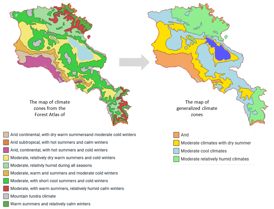 Figure 31A3-2. Generalization of climate zones for ES modeling
Հղումներ
38. Interactive Forest Atlas of Armenia. Available online: https://forestatlas.am (accessed on 26 June 2025).
39. HydroSHEDS. Seamless Hydrographic Data for Global and Regional Applications. Available online: https://hydrosheds.org (accessed on 26 June 2025).
40. ESRI Land Cover. Sentinel-2 10-Meter Land Use/Land Cover. Available online: https://livingatlas.arcgis.com/landcover (accessed on 26 June 2025).
41. ARMSTAT. Statistical Committee Republic of Armenia. Regional Statistics. Available online: https://armstat.am/en/?nid=651 (accessed on 26 June 2025).
42. Natural Capital Project. InVEST. Available online: https://naturalcapitalproject.stanford.edu/software/invest (accessed on 26 June 2025).
43. Ecoportal Armenia. River Basin Management Plans. Available online: https://ecoportal.am/en/river-basin-management-plans (accessed on 26 August 2025).
44. The United States Department of Agriculture’s Natural Resources Conservation Service. Part 630 Hydrology National Engineering Handbook. Chapter 7 Hydrologic Soil Groups; The United States Department of Agriculture’s Natural Resources Conservation Service: Washington, DC, USA, 2009. Available online: https://directives.nrcs.usda.gov/sites/default/files2/1712930597/11905.pdf (accessed on 26 June 2025).
45. Ecosystem accounting of Armenia. Web GIS of the Projet “Ecosystem Accounting in Armenia: Setting the Scene”. Available online: https://bccarmenia.nextgis.com (accessed on 26 June 2025).
46. Copernicus DEM—Global and European Digital Elevation Model. Available online: https://dataspace.copernicus.eu/explore-data/data-collections/copernicus-contributing-missions/collections-description/COP-DEM (accessed on 3 September 2025).
47. WorldClim. Global Climate and Weather Data. Available online: https://www.worldclim.org/data/index.html (accessed on 26 June 2025).
48. Weather in Armenia. Available online: http://armenia.pogoda360.ru (accessed on 26 June 2025).
49. BCC-Armenia. ES of Seasonal Water Flow Regulation (InVEST Seasonal Water Yield model). Available online: https://biodiversity-armenia.am/en/seea-ea/ongoing-projects/preliminary-results-on-ea/seasonal-water-yield (accessed on 26 June 2025).
50. Global Aridity and PET database. Available online: https://cgiarcsi.community/data/global-aridity-and-pet-database (accessed on 26 June 2025).
51. FAO. Chapter 6. Etc. Single Crop Coefficient (Kc). Available online: https://www.fao.org/4/X0490E/x0490e0b.htm (accessed on 26 June 2025).
52. FAO. Chapter 11. ETc During non-Growing Periods. Available online: https://www.fao.org/4/x0490e/x0490e0h.htm#frozen%20or%20snow%20covered%20surfaces (accessed on 26 June 2025).
53. FAO. Earth Observation. Country Indicators. Available online: https://www.fao.org/giews/earthobservation/country/index.jsp?code=ARM# (accessed on 26 June 2025).
54. Copernicus. Leaf Area Index. Available online: https://land.copernicus.eu/en/products/vegetation/leaf-area-index-300m-v1.0 (accessed on 26 June 2025).
55. Asante, K.O.; Artan, G.A.; Pervez, S.; Bandaragoda, C.; Verdin, J.P. Technical Manual for the Geospatial Stream Flow Model (GeoSFM); U.S. Geological Survey Open-File Report 2007–1441; USGS: Reston, VA, USA, 2008. Available online: https://pubs.usgs.gov/of/2007/1441/pdf/ofr2008-1441.pdf (accessed on 26 June 2025).
56. Hong, Y.; Adler, R.F. Estimation of global SCS curve numbers using satellite remote sensing and geospatial data. Int. J. Remote Sens. 2008, 29, 471–477. https://doi.org/10.1080/01431160701264292.
57. United States Department of Agriculture. Natural Resources Conservation Service. Urban Hydrology for Small Watersheds. Technical Release 55 (TR-55). 1986. Available online: https://www.nrc.gov/docs/ML1421/ML14219A437.pdf (accessed on 3 September 2025).
58. Panagos, P.; Borrelli, P.; Meusburger, K.; Alewell, C.; Lugato, E.; Montanarella, L. Estimating the soil erosion cover-management factor at the European scale. Land Use Policy 2015, 48, 38–50. https://doi.org/10.1016/j.landusepol.2015.05.021.
59. Joint Research Centre. European Soil Data Centre (ESDAC). Global Rainfall Erosivity. Available online: https://esdac.jrc.ec.europa.eu/content/global-rainfall-erosivity (accessed on 26 June 2025).
60. Allen, R.G.; Pruitt, W.O.; Raes, D.; Smith, M.; Pereira, L.S. Estimating Evaporation from Bare Soil and the Crop Coefficient for the Initial Period Using Common Soils Information. J. Irrig. Drain. Eng. 2005, 131, 14–23. https://doi.org/10.1061/(ASCE)0733-9437(2005)131:1(14).